Logistic Regression with Jupyter Notebook Link to heading

2. Model Implementation Link to heading

Choosing the Algorithm Link to heading

Use LogisticRegression from sklearn.linear_model.

from sklearn.linear_model import LogisticRegression

# Initialize the Logistic Regression model
model = LogisticRegression(max_iter=200)

Defining the Model Link to heading

Specify parameters such as C, solver, and max_iter. (This is optional for the first turn. We will focus on it later in Hyperparameter Tuning.)

Training the Model Link to heading

Fit the model using the training data.

# Train the model
model.fit(X_train, y_train)

Evaluating the Model Link to heading

Use metrics like accuracy, precision, and recall.

from sklearn.metrics import accuracy_score, classification_report, confusion_matrix

# Make predictions on the test set
y_pred = model.predict(X_test)

# Evaluate the model
print("Accuracy:", accuracy_score(y_test, y_pred))
print("Classification Report:\n", classification_report(y_test, y_pred))
print("Confusion Matrix:\n", confusion_matrix(y_test, y_pred))

Accuracy: 0.8636363636363636
Classification Report:
               precision    recall  f1-score   support

         0.0       1.00      1.00      1.00        13
         1.0       0.64      0.78      0.70         9
         2.0       0.90      0.82      0.86        22

    accuracy                           0.86        44
   macro avg       0.85      0.87      0.85        44
weighted avg       0.88      0.86      0.87        44

Confusion Matrix:
 [[13  0  0]
 [ 0  7  2]
 [ 0  4 18]]

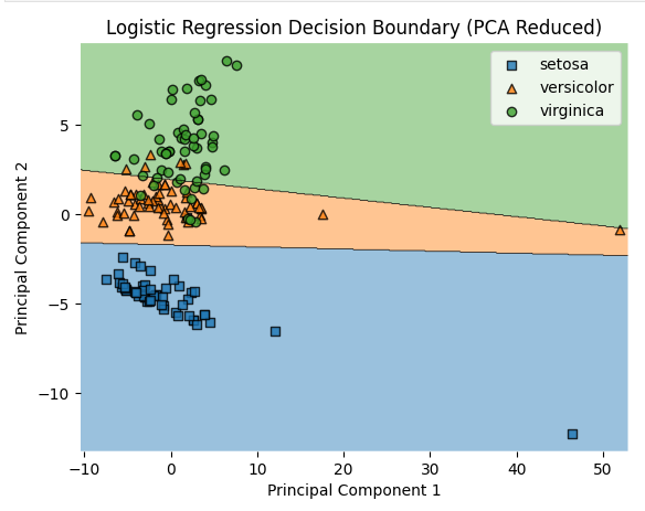
Visualizing Results Link to heading

Plot decision boundaries and confusion matrices.

import numpy as np
import matplotlib.pyplot as plt
from mlxtend.plotting import plot_decision_regions
from sklearn.decomposition import PCA
from sklearn.linear_model import LogisticRegression

# Perform PCA to reduce the dimensionality of the feature set to 2
pca = PCA(n_components=2)
X_train_pca = pca.fit_transform(X_train)  # Fit and transform the training data
X_test_pca = pca.transform(X_test)  # Transform the test data

# Initialize and train the logistic regression model on the PCA-reduced data
model_pca = LogisticRegression(max_iter=200)
model_pca.fit(X_train_pca, y_train)

# Plot decision regions using the PCA-reduced data
plot_decision_regions(X_train_pca, y_train.values.astype(np.int_), clf=model_pca, legend=2)
plt.xlabel('Principal Component 1')
plt.ylabel('Principal Component 2')
plt.title('Logistic Regression Decision Boundary (PCA Reduced)')

# Custom legend with actual class names
handles, labels = plt.gca().get_legend_handles_labels()
plt.legend(handles, ['setosa', 'versicolor', 'virginica'], frameon=True, loc='upper right')

plt.show()

Logistic Regression Decision Boundary (PCA Reduced)