Logistic Regression with Jupyter Notebook Link to heading
This part of the series demonstrates how to implement logistic regression on the Iris dataset using Jupyter Notebook. Jupyter Notebook provides an interactive environment for data analysis and visualization, making it a popular choice for data scientists.
1. Dataset Preparation Link to heading
Loading the Dataset Link to heading
We will use the Iris dataset, a well-known dataset for classification tasks. It is available in the sklearn library.
# Import necessary libraries
from scipy import stats
import numpy as np
import pandas as pd
from sklearn.datasets import load_iris
import seaborn as sns
import matplotlib.pyplot as plt

# Load the original Iris dataset
iris = load_iris()
X_original = pd.DataFrame(iris.data, columns=iris.feature_names)
y_original = pd.Series(iris.target, name='target')

# Original Iris datasaet
data_original = pd.DataFrame(data=iris.data, columns=iris.feature_names)
data_original['target'] = iris.target
print(f"Number of rows in the original dataset: {len(data_original)}")
data_original.info()
As the original Iris dataset is very clean, we want to add some artificial noise to it to perform data cleaning tasks. This is not usually the case of the data preparation process, and the noise is added only for presentation purposes.
- Artificial Noise Addition: The clean nature of the Iris dataset makes it unsuitable for demonstrating data cleaning tasks. Therefore, synthetic data is added to simulate scenarios where data cleaning is necessary.
- Combination Purpose: The combination of datasets is purely for presentation and educational purposes, emphasizing techniques that may be needed in real-world data preparation processes.
# Step 1: Extend the dataset using SMOTE (Synthetic Minority Over-sampling Technique)
# SMOTE generates synthetic samples to balance the dataset, which can help in training
# models with imbalanced data. Here, SMOTE is used to generate additional synthetic data
# for demonstration purposes, not because of class imbalance.
smote = SMOTE(sampling_strategy='auto', random_state=42)
X_generated, y_generated = smote.fit_resample(X_original, y_original)

# Step 2: Create a DataFrame from the generated data
# The synthetic data is converted back into a DataFrame to resemble the structure of the original dataset.
data_generated = pd.DataFrame(X_generated, columns=iris.feature_names)
data_generated['target'] = y_generated

# Step 3: Combine the original and generated datasets
# The generated synthetic data is combined with the original clean dataset to introduce
# artificial noise. This combination is only for presentation purposes, showcasing
# data cleaning and preprocessing steps.
data = pd.concat([X_original.assign(target=y_original), data_generated], ignore_index=True)

# Step 4: Introduce missing values (20% of the data)
# Randomly set 20% of the values in the dataset to NaN
missing_rate = 0.2
missing_mask = np.random.rand(*data.shape) < missing_rate
data = data.mask(missing_mask)

# Step 5: Introduce outliers (10% of the data)
# Randomly select 10% of the rows and add outliers by multiplying by a random factor
outlier_rate = 0.1
num_outliers = int(outlier_rate * len(data))
outlier_indices = np.random.choice(data.index, num_outliers, replace=False)

# Add outliers by modifying the data at the selected indices
data.loc[outlier_indices, data.columns[:-1]] *= \
    np.random.uniform(1.5, 3.0, size=(num_outliers, len(data.columns) - 1))
Exploring the Data Link to heading
# Display the extended dataset with missing values and outliers
data.info()
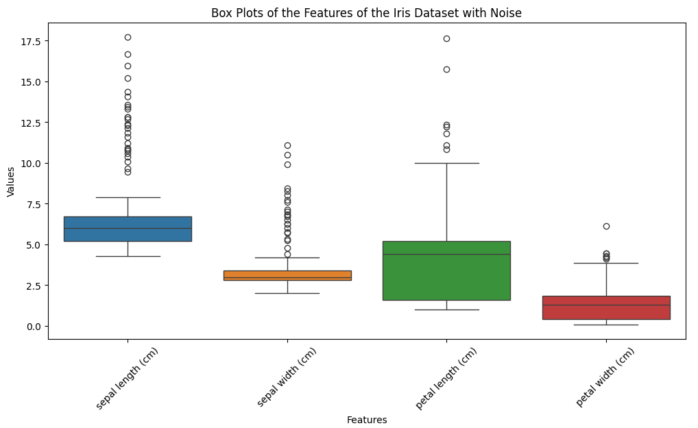
# Plotting box plots for each feature
plt.figure(figsize=(12, 6))
sns.boxplot(data=data.drop(columns=['target']))
plt.title('Box Plots of the Features of the Iris Dataset with Noise')
plt.xlabel('Features')
plt.ylabel('Values')
plt.xticks(rotation=45)
plt.show()
RangeIndex: 300 entries, 0 to 299
Data columns (total 5 columns):
 #   Column             Non-Null Count  Dtype
---  ------             --------------  -----
 0   sepal length (cm)  250 non-null    float64
 1   sepal width (cm)   238 non-null    float64
 2   petal length (cm)  236 non-null    float64
 3   petal width (cm)   247 non-null    float64
 4   target             239 non-null    float64
dtypes: float64(5)
memory usage: 11.8 KB
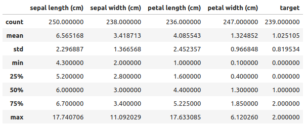
data.describe(include="all")
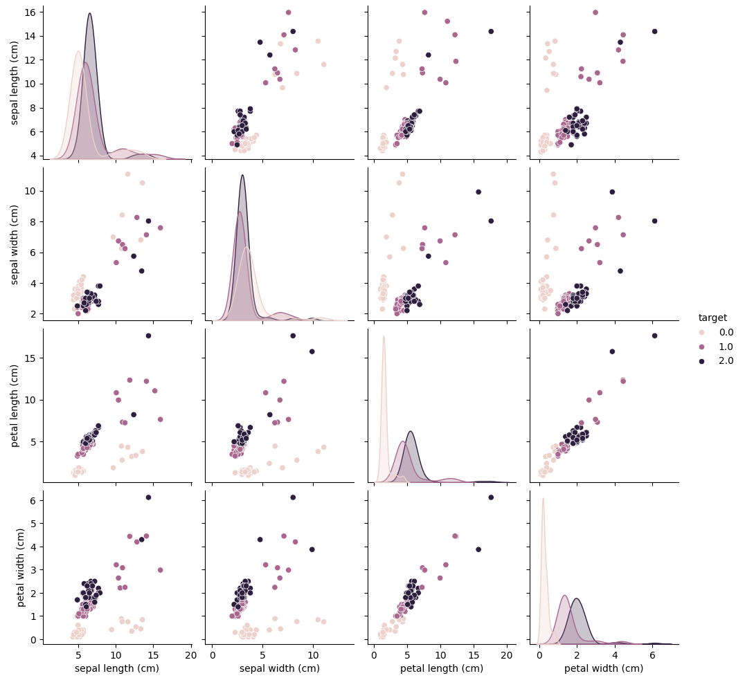
Use pandas and seaborn for data exploration and visualization.
# Pairplot to visualize the data
sns.pairplot(data, hue='target')
plt.show()
Data Cleaning Link to heading
Handle any missing values or outliers (the Iris dataset is clean, so this step is often skipped).
Handling Missing Values: Link to heading
In many real-world datasets, missing values are common. You can handle them by either removing rows/columns with missing values or filling them with appropriate values (imputation).
# Check for missing values
# Explanation: This line checks for missing values in the dataset by counting
# the number of NaN values in each column. Understanding the extent of missing data
# helps in deciding how to handle these gaps appropriately.
print("Missing values by feature before cleaning:")
print(data.isnull().sum())

# Remove rows where the 'target' value is not in [0, 1, 2]
# Purpose: This step removes rows where the target column does not have
# valid classification values (0, 1, 2), which represent the three species
# in the Iris dataset (Setosa, Versicolor, and Virginica).
# Reason for Cleanup: Rows with invalid or missing target values can negatively
# impact model training, as they introduce noise that does not contribute to learning
# the correct classification patterns. Removing these rows ensures the dataset
# only contains relevant data that directly supports accurate training.
data.drop(data[~data['target'].isin([0, 1, 2])].index, inplace=True)

# Fill missing values with the mean of each column directly in the original dataset
# Purpose: This line fills any missing values in the dataset with the mean
# of their respective columns.
# Reason for Cleanup:
# Handling Partial Data: If only a single feature is missing in a row,
# it would be wasteful to discard the entire row, as the other feature
# values still provide useful information for training.
# Preserving Dataset Integrity: Using the mean value allows the model
# to retain as much data as possible while maintaining a balanced approach,
# which can enhance model performance and stability.
# Minimizing Bias: Filling missing values with the mean helps to maintain
# the statistical properties of the dataset, ensuring that the model remains
# unbiased towards any specific values that could be introduced
# by more complex imputation techniques.
data.fillna(data.mean(), inplace=True)

print("\nMissing values by feature after cleaning:")
print(data.isnull().sum())

# Display the cleaned dataset
data_cleaned.head()
Missing values by Feature before cleaning:
sepal length (cm)    0
sepal width (cm)     0
petal length (cm)    0
petal width (cm)     0
target               0
dtype: int64

Missing values by Feature after cleaning:
sepal length (cm)    0
sepal width (cm)     0
petal length (cm)    0
petal width (cm)     0
target               0
dtype: int64
Handling Outliers: Link to heading
Outliers can skew the results of your model. You can detect outliers using statistical methods or visualization and handle them by removing or transforming them.
# Detect outliers using Z-score, but don't modify the target column
z_scores = np.abs(stats.zscore(data.drop(columns=['target'])))
# Remove rows with outliers directly in the original dataset
data = data[(z_scores < 2.5).all(axis=1)]
# Display the dataset after outlier removal
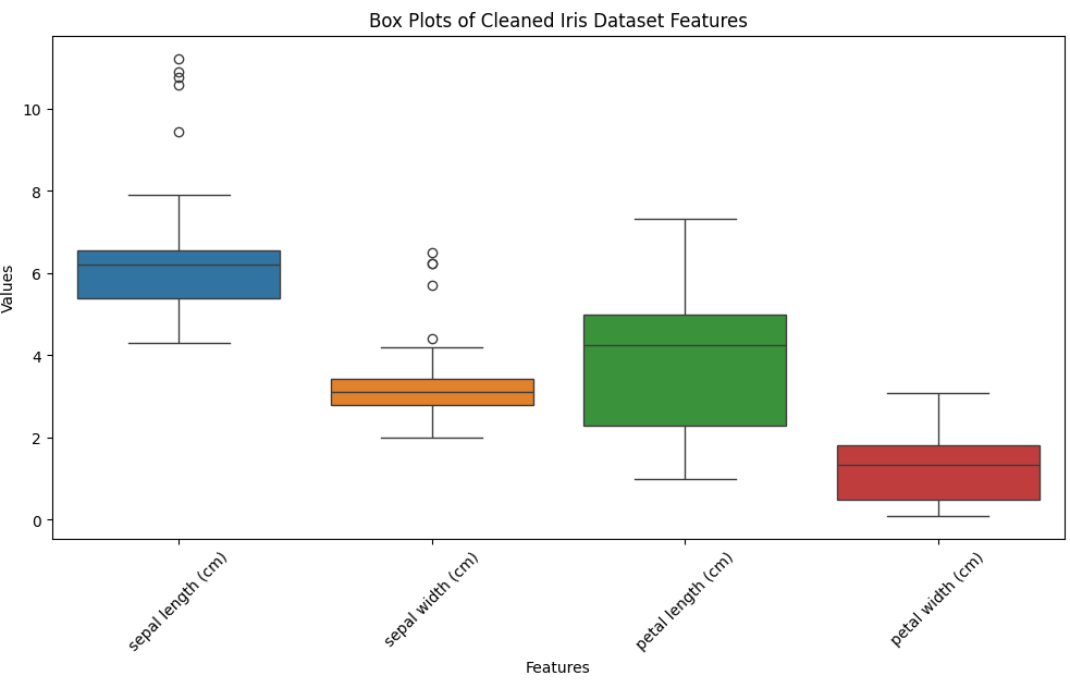
# Plotting box plots for each feature
plt.figure(figsize=(12, 6))
sns.boxplot(data=data.drop(columns=['target']))
plt.title('Box Plots of Cleaned Iris Dataset Features')
plt.xlabel('Features')
plt.ylabel('Values')
plt.xticks(rotation=45)
plt.show()
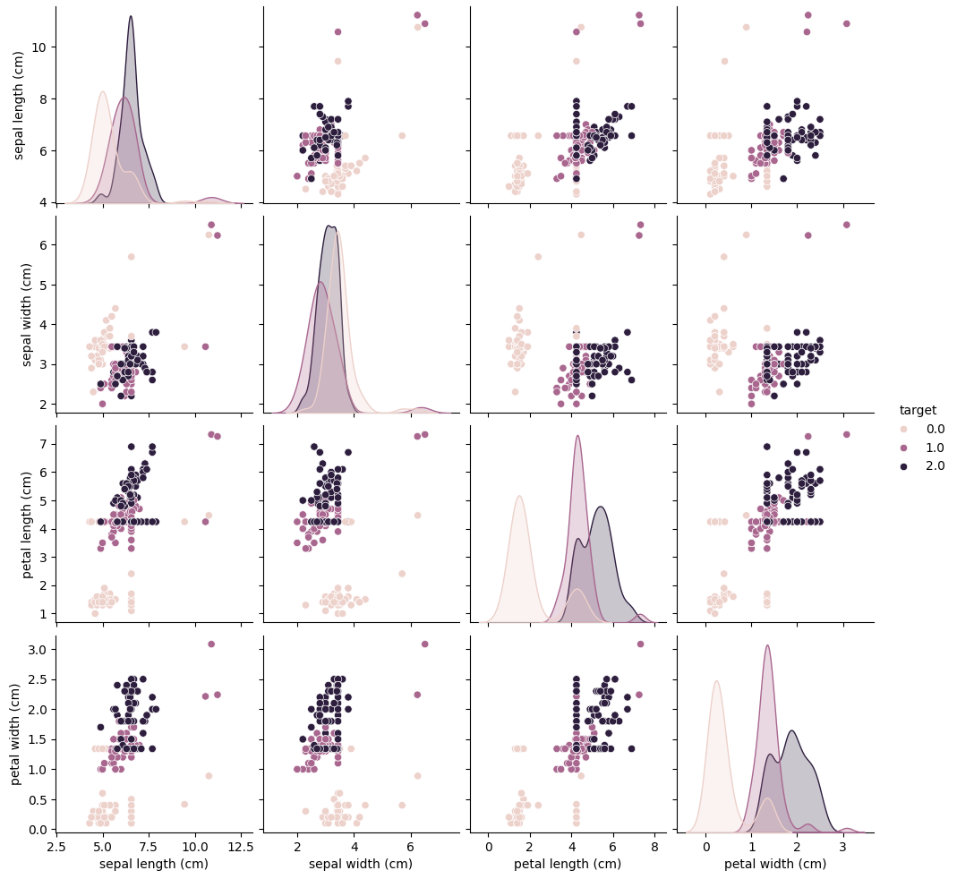
# Pairplot after cleaning the data
sns.pairplot(data, hue='target')
plt.show()
Feature Engineering Link to heading
Feature engineering involves transforming raw data into features that better represent the underlying problem to the predictive models, resulting in improved model accuracy. Here, we will modify or create features for the dataset.
- Creating Interaction Terms: Interaction terms can capture the interaction between features.
# Creating interaction terms
data['sepal length * sepal width'] = data['sepal length (cm)'] * data['sepal width (cm)']
data['petal length * petal width'] = data['petal length (cm)'] * data['petal width (cm)']
- Feature Transformation: Apply mathematical transformations to features.
# Applying logarithmic transformation
data['log sepal length'] = np.log(data['sepal length (cm)'])
- Normalization: Scale features to a similar range.
from sklearn.preprocessing import MinMaxScaler

# Normalizing features
scaler = MinMaxScaler()
data[['sepal length (cm)', 'sepal width (cm)', 'petal length (cm)', 'petal width (cm)']] = scaler.fit_transform(
    data[['sepal length (cm)', 'sepal width (cm)', 'petal length (cm)', 'petal width (cm)']]
)
These steps enhance the features, making them more suitable for machine learning algorithms and improving model performance.
Splitting the Data Link to heading
Use train_test_split from sklearn.model_selection to divide the dataset.
from sklearn.model_selection import train_test_split

# Mapping numerical target values to class names
target_mapping = {0: 'setosa', 1: 'versicolor', 2: 'virginica'}
data['target_name'] = data['target'].map(target_mapping)


# Split the dataset into training and testing sets
X_train, X_test, y_train, y_test = train_test_split(
    data.drop(columns=['target', 'target_name']),
    data['target'],
    test_size=0.2,
    random_state=42
)